Design Specification: Condition-Specific Parameters (Speed–Accuracy Tradeoff) |

View the notebook on GitHub

This tutorial demonstrates how to implement design specifications in JEAM—that is, how experimental manipulations are translated into condition-specific model parameters within a single likelihood function.

In the example below (based on the accompanying notebook), we fit a Circular Diffusion Model (CDM) to data from an orientation judgment task reported in Kvam (2019). In this task, participants viewed a dynamic Gabor patch and reported the average orientation of the stimulus by clicking on a circular response scale:

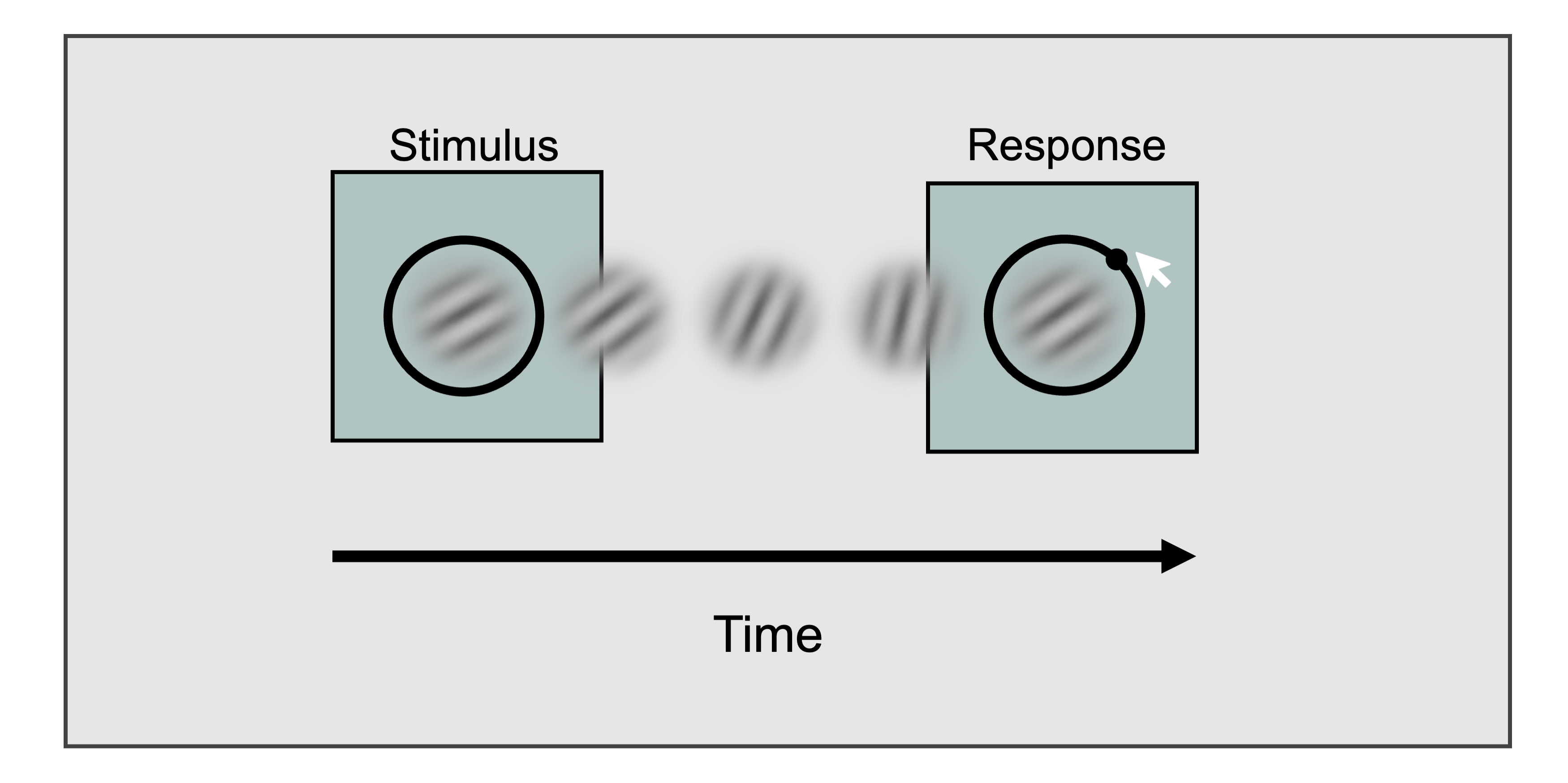
The experimental design includes two orthogonal manipulations:

• a speed–accuracy trade-off instruction (isSpeed),
• a stimulus difficulty manipulation (jitter ∈ {15, 30, 45} degrees).

To model these data, we specify a circular diffusion model with the following structure:

• the decision threshold is condition-specific, differing between speed and accuracy blocks;
• the drift magnitude varies across difficulty levels (indexed by jitter);
• the drift angle and non-decision time (NDT) are shared across all conditions.

This parameterization allows the model to capture systematic changes in response caution and evidence quality induced by task instructions and stimulus difficulty, while maintaining a parsimonious representation of shared decision dynamics.

---

1. Import required packages

import numpy as np
import pandas as pd

from tqdm import tqdm

import seaborn as sns
import matplotlib.pyplot as plt

from scipy.optimize import differential_evolution

from jeam.utility.datasets import load_kvam2019
from jeam.Models.Circular import CircularDiffusionModel as CDM

---

2. Load the dataset

data = load_kvam2019()

data.head()

Participant	isSpeed	jitter	response	deviation	rt
100	0	45	1.9217	-0.5391	1.2595
100	0	30	1.7845	0.32968	0.86939
100	0	15	0.26625	-0.30658	0.8009
100	0	30	2.157	0.15855	1.0019
100	0	15	1.7277	0.0072374	2.364

This dataset includes:

• Participant: participant identifier,
• isSpeed: instruction condition (1 = speed, 0 = accuracy),
• jitter: stimulus difficulty (15, 30, 45 degrees),
• deviation: signed angular response deviation (radians),
• rt: response time (seconds).

---

3. Define the likelihood with design-specific parameters

The likelihood function below constructs trial-wise drift vectors based on the experimental design and routes trials to condition-specific thresholds depending on the instruction condition.

Model specification

• Two decision thresholds: threshold_speed and threshold_accuracy
• One non-decision time: ndt
• One drift direction: parameterized by a drift angle drift_angle
• Three drift magnitudes: one per jitter level (15, 30, 45)

def negative_log_likelihood(params, rt, theta, isSpeed, jitter, model):
    threshold_speed = params[0]
    threshold_accuracy = params[1]
    ndt = params[2]
    drift_angle = params[3]

    # Drift direction is shared across conditions
    drift_direction = np.array([np.cos(drift_angle), np.sin(drift_angle)])

    # Drift magnitude depends on jitter
    drift_magnitudes = np.empty(rt.shape)
    drift_magnitudes[jitter == 15] = params[4]
    drift_magnitudes[jitter == 30] = params[5]
    drift_magnitudes[jitter == 45] = params[6]

    # Trial-wise drift vectors
    drift_vectors = np.outer(drift_magnitudes, drift_direction)

    # Condition-specific thresholds (speed vs accuracy)
    logpdf_speed = model.joint_lpdf(
        rt[isSpeed == 1],
        theta[isSpeed == 1],
        drift_vectors[isSpeed == 1, :],
        ndt,
        threshold_speed,
    )

    logpdf_accuracy = model.joint_lpdf(
        rt[isSpeed == 0],
        theta[isSpeed == 0],
        drift_vectors[isSpeed == 0, :],
        ndt,
        threshold_accuracy,
    )

    return -np.sum(logpdf_speed) - np.sum(logpdf_accuracy)

---

4. Set parameter bounds and fit the model per participant

param_names = ['threshold_speed', 
               'threshold_accuracy',
               'ndt', 
               'drift_angle',
               'drift_magnitude15',
               'drift_magnitude30',
               'drift_magnitude45']


# Parameter bounds
bounds = [
    (0.05, 5.0),   # threshold speed
    (0.05, 5.0),   # threshold accuracy
    (0.0, 1.0),    # non-decision time
    (-np.pi, np.pi),    # drift angle
    (0, 8.0),   # drift magnidute (length) for jitter=15
    (0, 8.0),   # drift magnidute (length) for jitter=30
    (0, 8.0),   # drift magnidute (length) for jitter=45
]

model = CDM(threshold_dynamic="fixed")

estimation_rows = []

# Estimate model parameters separately for each participant
for sbj in tqdm(data.Participant.unique()):
    sbj_data = data[data['Participant']==sbj].reset_index(drop=True)

    # Optimize the negative log-likelihood function
    result = differential_evolution(
                negative_log_likelihood,
                bounds=bounds,
                args=(sbj_data["rt"].values, 
                      sbj_data["deviation"].values,
                      sbj_data["isSpeed"].values,
                      sbj_data["jitter"].values, model),
    )

    k = len(result.x) # number of free parameters
    n = sbj_data.shape[0] # number of trials for the participant
    nlpdf = result.fun # optimized negative log-likelihood value

    # store the goodness of fit criterion and estimated parameters for each subject
    row = {
        "Participant": sbj, 
        "nlpdf": nlpdf, 
        "AIC": 2 * nlpdf + 2 * k, 
        "BIC": 2 * nlpdf + k * np.log(n)
    }
    row.update(dict(zip(param_names, result.x)))

    estimation_rows.append(row)

100%|███████████████████████████████████████████| 12/12 [00:12<00:00,  1.06s/it]

estimation_data = pd.DataFrame(estimation_rows)
estimation_data

Participant	nlpdf	AIC	BIC	threshold_speed	threshold_accuracy	ndt	drift_angle	drift_magnitude15	drift_magnitude30	drift_magnitude45
100	335.535	685.07	715.837	0.866757	1.50936	0.440777	-0.0157439	3.59821	2.76672	1.54547
101	283.352	580.704	609.877	1.0362	1.33893	0.416766	-0.0199686	3.94078	2.66761	1.40861
110	557.592	1129.18	1158.34	0.978971	1.27506	0.337027	0.0578871	2.92682	1.52246	0.730462
120	471.097	956.194	985.189	0.905203	1.53838	0.362234	0.0143186	2.69224	1.7259	1.05211
130	248.978	511.956	541.172	0.715614	0.889673	0.2799	0.0284188	3.0901	2.15851	1.09002
140	93.2438	200.488	229.704	0.999547	1.04782	0.388389	0.00383741	4.87936	3.23159	1.58084
150	196.158	406.315	435.532	0.917433	0.870011	0.332569	0.0459289	3.89978	2.50724	1.43862
170	282.323	578.647	607.805	0.835069	1.09277	0.254983	0.0846156	3.43038	2.25192	1.16668
180	462.984	939.967	969.11	0.971128	1.69997	0.258889	-0.127637	2.87725	2.02574	1.12141
190	277.391	568.781	597.639	0.840641	1.94945	0.316306	-0.0698122	3.43441	2.26668	1.34496
200	427.305	868.61	897.619	0.883803	1.09596	0.232506	0.0471421	2.91083	2.05821	1.05827
210	303.888	621.777	650.876	0.894596	1.1362	0.368374	-0.0905744	3.27711	2.2957	1.26796

---

5. Model-based prediction (posterior predictive simulation)

We next perform posterior predictive simulations using the fitted parameters. By comparing summary statistics from the observed data and model-generated data, we assess whether the model captures systematic effects of task instructions and stimulus difficulty.

n_sample_condition = 200
predictions = []

for sbj in tqdm(data.Participant.unique()):
    # model's parameters for each subject
    prms = estimation_data[estimation_data["Participant"] == sbj].iloc[0]

    drift_dir = np.array([np.cos(prms["drift_angle"]), 
                          np.sin(prms["drift_angle"])])

    for jitter in [15, 30, 45]:
        drift_mag = prms[f"drift_magnitude{jitter}"]
        drift_vec = drift_mag * drift_dir

        # Speed condition
        speed_df = model.simulate(
            drift_vec,
            prms["ndt"],
            threshold=prms["threshold_speed"],
            n_sample=n_sample_condition,
        )
        speed_df["isSpeed"] = 1
        speed_df["jitter"] = jitter
        speed_df["Participant"] = sbj

        # Accuracy condition
        acc_df = model.simulate(
            drift_vec,
            prms["ndt"],
            threshold=prms["threshold_accuracy"],
            n_sample=n_sample_condition,
        )
        acc_df["isSpeed"] = 0
        acc_df["jitter"] = jitter
        acc_df["Participant"] = sbj

        predictions.append(pd.concat([speed_df, acc_df], ignore_index=True))

model_prediction = pd.concat(predictions, ignore_index=True)
model_prediction.head()

100%|███████████████████████████████████████████| 12/12 [00:02<00:00,  4.92it/s]

rt	response	isSpeed	jitter	Participant
0.662777	0.270706	1	15	100
0.578777	-0.612121	1	15	100
0.568777	0.182161	1	15	100
0.661777	-0.752912	1	15	100
0.714777	-0.727197	1	15	100

6. Compare summary measures

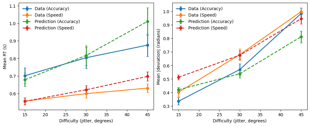
A common approach is to compare mean RT and mean absolute deviation across conditions:

data_plot = data.copy()
data_plot["abs_dev"] = np.abs(data_plot["deviation"])

pred_plot = model_prediction.copy()
pred_plot["abs_dev"] = np.abs(pred_plot["response"])

# Helper: compute mean + SEM
def summarize(df, value_col, source_name):
    g = (
        df.groupby(["jitter", "isSpeed"])[value_col]
        .agg(mean="mean", sem="sem")
        .reset_index()
    )
    g["source"] = source_name
    g["metric"] = value_col
    return g

def plot_metric(ax, metric, ylabel):
    sub = summary[summary["metric"] == metric].copy()

    # plot each (source × condition) as a separate line with error bars
    for (source, condition), sdf in sub.groupby(["source", "condition"]):
        sdf = sdf.sort_values("jitter")
        ax.errorbar(
            sdf["jitter"],
            sdf["mean"],
            yerr=sdf["sem"],
            marker="o",
            linewidth=2,
            linestyle="-" if source == "Data" else "--",
            label=f"{source} ({condition})",
            capsize=3,
        )

    ax.set_xlabel("Difficulty (jitter, degrees)")
    ax.set_ylabel(ylabel)
    ax.legend(frameon=False)

summary = pd.concat(
    [
        summarize(data_plot, "rt", "Data"),
        summarize(data_plot, "abs_dev", "Data"),
        summarize(pred_plot, "rt", "Prediction"),
        summarize(pred_plot, "abs_dev", "Prediction"),
    ],
    ignore_index=True,
)

summary["condition"] = summary["isSpeed"].map({0: "Accuracy", 1: "Speed"})
summary["jitter"] = summary["jitter"].astype(int)

We focus on two key summary measures: mean response time, which indexes response speed, and mean absolute response deviation, which quantifies response precision. Together, these measures capture the speed–accuracy trade-off and characterize how task difficulty influences both response speed and response precision in continuous-report tasks.

fig, axes = plt.subplots(1, 2, figsize=(10, 4), constrained_layout=True)

plot_metric(axes[0], "rt", "Mean RT (s)")
plot_metric(axes[1], "abs_dev", "Mean |deviation| (radians)")

plt.show()

---

Notes

• This pattern—mapping design factors to different model parameters—scales to more complex designs (e.g., stimulus-specific drifts, participant-level covariates, hierarchical extensions).
• The key idea is to construct trial-wise parameters (like drift_vectors) and to route trials to condition-specific parameters (like thresholds) inside the likelihood.

---

References

Kvam, P. D. (2019). Modeling accuracy, response time, and bias in continuous orientation judgments. Journal of Experimental Psychology: Human Perception and Performance, 45(3), 301–318. https://doi.org/10.1037/xhp0000606