Collapsing Threshold Models: A Parameter Recovery Simulation |

View the notebook on GitHub

This tutorial illustrates how to use JEAM to fit collapsing threshold diffusion models and to fit a joint model on observed data from multiple sources (e.g., behavior and neural signals).

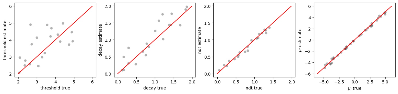
This tutorial contains a simple parameter recovery study using Circular Diffusion Model (CDM) with a linear collapsing decision threshold. We considered two setups for parameter recovery:

Uninformed collapsing-threshold model: fit the model using only choice/RT data.
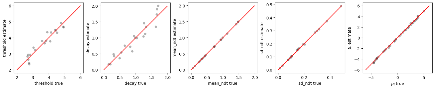
NDT-informed collapsing-threshold model (joint modeling): fit the model using choice/RT data and additional measurements that inform the non-decision time (NDT) distribution.

Import required packages

import numpy as np
import pandas as pd
from tqdm import tqdm

import seaborn as sns
import matplotlib.pyplot as plt

from scipy.optimize import differential_evolution

from jeam.Models.Circular import CircularDiffusionModel as CDM

1. Uninformed collapsing threshold diffusion models:

In the first setup, we simulate data from a CDM with a linear collapsing threshold and then recover:

threshold: initial decision threshold,
decay: collapse rate (linear),
ndt: non-decision time,
mu_x, mu_y: drift vector components.

1.1 Negative log-likelihood

def negative_log_likelihood(params, rt, theta, model):
    threshold = params[0]            # initial decision threshold
    decay = params[1]                # decay rate of threshold
    ndt = params[2]                  # non-decision time
    drift_vec = np.array([params[3], params[4]])  # drift vector

    logpdf = model.joint_lpdf(rt, theta, drift_vec, ndt, threshold, decay=decay)

    return -np.sum(logpdf)

1.2 Simulation setup

n_trials = 500

recovery_df = {
    "threshold_true": [], "threshold_estimate": [],
    "decay_true": [], "decay_estimate": [],
    "ndt_true": [], "ndt_estimate": [],
    "mu_x_true": [], "mu_x_estimate": [],
    "mu_y_true": [], "mu_y_estimate": []
}

# Bounds for estimation
min_threshold, max_threshold = 2, 5
min_decay, max_decay = 0.05, 2
min_ndt, max_ndt = 0, 1.5
min_mu, max_mu = -5, 5

prms_bounds = [
    (min_threshold, max_threshold),
    (min_decay, max_decay),
    (min_ndt, max_ndt),
    (min_mu, max_mu),
    (min_mu, max_mu),
]

model = CDM(threshold_dynamic='exponential')

1.3 Simulation and estimation loop

for n in tqdm(range(20)):
    # Random generative parameters
    threshold = np.random.uniform(min_threshold, max_threshold)
    decay = np.random.uniform(min_decay, max_decay)
    mu_x = np.random.uniform(min_mu, max_mu)
    mu_y = np.random.uniform(min_mu, max_mu)
    drift_vector = np.array([mu_x, mu_y])
    ndt = np.random.uniform(min_ndt, max_ndt)

    # Simulating data with random generated parameters
    sim_df = model.simulate(
        drift_vector,
        ndt,
        threshold,
        decay=decay,
        n_sample=n_trials,
    )

    # Estimate parameters
    min_ans = differential_evolution(
        negative_log_likelihood,
        bounds=prms_bounds,
        args=(sim_df["rt"].values, sim_df["response"].values, model),
    )

    # Store true parameters
    recovery_df["threshold_true"].append(threshold)
    recovery_df["decay_true"].append(decay)
    recovery_df["ndt_true"].append(ndt)
    recovery_df["mu_x_true"].append(mu_x)
    recovery_df["mu_y_true"].append(mu_y)

    # Store estimates
    recovery_df["threshold_estimate"].append(min_ans.x[0])
    recovery_df["decay_estimate"].append(min_ans.x[1])
    recovery_df["ndt_estimate"].append(min_ans.x[2])
    recovery_df["mu_x_estimate"].append(min_ans.x[3])
    recovery_df["mu_y_estimate"].append(min_ans.x[4])

100%|█████████████████████████████████████████| 20/20 [03:01<00:00,  9.07s/it]

plt.figure(figsize=(13, 3), layout="constrained")

plt.subplot(141)
plt.plot(np.arange(2, 6, 0.01), np.arange(2, 6, 0.01), c="red")
sns.scatterplot(x="threshold_true", y="threshold_estimate", data=recovery_df, color="black", alpha=0.3)
plt.xlabel("threshold true")
plt.ylabel("threshold estimate")

plt.subplot(142)
plt.plot(np.arange(0, 2, 0.01), np.arange(0, 2, 0.01), c="red")
sns.scatterplot(x="decay_true", y="decay_estimate", data=recovery_df, color="black", alpha=0.3)
plt.xlabel("decay true")
plt.ylabel("decay estimate")

plt.subplot(143)
plt.plot(np.arange(0, 2, 0.01), np.arange(0, 2, 0.01), c="red")
sns.scatterplot(x="ndt_true", y="ndt_estimate", data=recovery_df, color="black", alpha=0.3)
plt.xlabel("ndt true")
plt.ylabel("ndt estimate")

plt.subplot(144)
plt.plot(np.arange(-6, 6, 0.01), np.arange(-6, 6, 0.01), c="red")
sns.scatterplot(x="mu_x_true", y="mu_x_estimate", data=recovery_df, color="black", alpha=0.3)
sns.scatterplot(x="mu_y_true", y="mu_y_estimate", data=recovery_df, color="black", alpha=0.3)
plt.xlabel(r"$\mu_i$ true")
plt.ylabel(r"$\mu_i$ estimate")
plt.show()

png

2. NDT-informed collapsing threshold diffusion models (joint modeling):

In many experiments, additional measurements can constrain the NDT distribution (e.g., encoding time, motor time, or other process-pure measures). Here we demonstrate a simple joint model where:

the diffusion model explains choice/RT data,
a Gaussian measurement model explains observed ndt_measurements.

We recover:

threshold, decay,
mean_ndt and sd_ndt,
mu_x, mu_y.

2.1 Negative joint log-likelihood

def negative_log_likelihood_ndt_informed(params, rt, theta, ndt_mesurements, model):
    threshold =  params[0]    # initial decision threshold
    decay = params [1]        # decay rate of threshold

    # mean of non-decision time measurements (shared across observation and diffusion model)
    mean_ndt = params[2] 
    sd_ndt = params[3] # SD of non-decision time measurements
    drift_vec = np.array([params[4], params[5]]) # drift vector

    ndt_logpdf = -0.5 * (ndt_mesurements - mean_ndt)**2/sd_ndt**2 - 0.5 * np.log(2*np.pi*sd_ndt**2)
    choice_logpdf = model.joint_lpdf(rt, theta, drift_vec, mean_ndt, threshold, decay=decay)

    return -np.sum(choice_logpdf) - np.sum(ndt_logpdf)

2.2 Simulation setup

n_trials = 500

recovery_df = {
    "threshold_true": [], "threshold_estimate": [],
    "decay_true": [], "decay_estimate": [],
    "mean_ndt_true": [], "mean_ndt_estimate": [],
    "sd_ndt_true": [], "sd_ndt_estimate": [],
    "mu_x_true": [], "mu_x_estimate": [],
    "mu_y_true": [], "mu_y_estimate": []
}

min_threshold, max_threshold = 2, 5
min_decay, max_decay = 0.05, 2
min_mean_ndt, max_mean_ndt = 0.05, 1.5
min_sd_ndt, max_sd_ndt = 0.01, 0.5
min_mu, max_mu = -5, 5

prms_bounds = [
    (min_threshold, max_threshold),
    (min_decay, max_decay),
    (min_mean_ndt, max_mean_ndt),   
    (min_sd_ndt, max_sd_ndt),
    (min_mu, max_mu),
    (min_mu, max_mu),
]

model = CDM(threshold_dynamic='exponential')

2.3 Simulation and estimation loop

for n in tqdm(range(20)):    
    # generating some random parameters
    threshold = np.random.uniform(min_threshold, max_threshold)
    decay = np.random.uniform(min_decay, max_decay)
    mu_x = np.random.uniform(min_mu, max_mu)
    mu_y = np.random.uniform(min_mu, max_mu)
    drift_vector = np.array([mu_x, mu_y])

    mean_ndt = np.random.uniform(0.05, max_ndt)
    sd_ndt = np.random.uniform(mean_ndt/5, mean_ndt/3)
    ndt_mesurements = mean_ndt + sd_ndt*np.random.randn(n_trials)

    sim_df = model.simulate(drift_vector, 
                            mean_ndt,
                            threshold, 
                            decay=decay,
                            n_sample=n_trials)

    # Estimating the paramters for the simulated data
    min_ans = differential_evolution(negative_log_likelihood_ndt_informed, 
                                     args=(sim_df['rt'].values, 
                                           sim_df['response'].values,
                                           ndt_mesurements,
                                           model), 
                                     bounds=prms_bounds)


    # Storing the true generating parameters
    recovery_df['threshold_true'].append(threshold)
    recovery_df['decay_true'].append(decay)
    recovery_df['mean_ndt_true'].append(mean_ndt)
    recovery_df['sd_ndt_true'].append(sd_ndt)
    recovery_df['mu_x_true'].append(mu_x)
    recovery_df['mu_y_true'].append(mu_y)

    # Stroing the estimated parameters
    recovery_df['threshold_estimate'].append(min_ans.x[0])
    recovery_df['decay_estimate'].append(min_ans.x[1])
    recovery_df['mean_ndt_estimate'].append(min_ans.x[2])
    recovery_df['sd_ndt_estimate'].append(min_ans.x[3])
    recovery_df['mu_x_estimate'].append(min_ans.x[4])
    recovery_df['mu_y_estimate'].append(min_ans.x[5])

100%|█████████████████████████████████████████| 20/20 [03:49<00:00, 11.45s/it]

plt.figure(figsize=(15, 3), layout='constrained')

plt.subplot(151)
plt.plot(np.arange(2, 6, 0.01), np.arange(2, 6, 0.01), c='red')
sns.scatterplot(x='threshold_true', y='threshold_estimate', data=recovery_df, color='black', alpha=0.3);
plt.xlabel(r'threshold true')
plt.ylabel(r'threshold estimate')

plt.subplot(152)
plt.plot(np.arange(0, 2, 0.01), np.arange(0, 2, 0.01), c='red')
sns.scatterplot(x='decay_true', y='decay_estimate', data=recovery_df, color='black', alpha=0.3);
plt.xlabel(r'decay true')
plt.ylabel(r'decay estimate')

plt.subplot(153)
plt.plot(np.arange(0, 2, 0.01), np.arange(0, 2, 0.01), c='red')
sns.scatterplot(x='mean_ndt_true', y='mean_ndt_estimate', data=recovery_df, color='black', alpha=0.3);
plt.xlabel(r'mean_ndt true')
plt.ylabel(r'mean_ndt estimate')

plt.subplot(154)
plt.plot(np.arange(0, 0.5, 0.01), np.arange(0, 0.5, 0.01), c='red')
sns.scatterplot(x='sd_ndt_true', y='sd_ndt_estimate', data=recovery_df, color='black', alpha=0.3);
plt.xlabel(r'sd_ndt true')
plt.ylabel(r'sd_ndt estimate')

plt.subplot(155)
plt.plot(np.arange(-6, 6, 0.01), np.arange(-6, 6, 0.01), c='red')
sns.scatterplot(x='mu_x_true', y='mu_x_estimate', data=recovery_df, color='black', alpha=0.3);
sns.scatterplot(x='mu_y_true', y='mu_y_estimate', data=recovery_df, color='black', alpha=0.3);
plt.xlabel(r'$\mu_i$ true')
plt.ylabel(r'$\mu_i$ estimate');

png

Notes

Always check parameter recovery

When introducing a new mapping function, mixture model, or joint model, always perform a parameter recovery study before applying the model to empirical data.

Parameter recovery helps ensure that: - the likelihood function is implemented correctly, - parameters are identifiable given the data and design, - different model components (e.g., guessing vs. diffusion, threshold vs. NDT) are not confounded.

Skipping this step can lead to misleading parameter estimates and incorrect theoretical conclusions.

References

Hadian Rasanan, A. H., Schumacher, L., Nunez, M. D., Weindel, G., & Rieskamp, J. (2025). Non-decision time-informed collapsing threshold diffusion model: A joint modeling framework with identifiable time-dependent parameters. bioRxiv, 2025-10. https://doi.org/10.1101/2025.10.30.685574
Hadian Rasanan, A. H., Evans, N. J., Amani Rad, J., & Rieskamp, J. (2025). Parameter estimation of hyper-spherical diffusion models with a time-dependent threshold: An integral equation method. Behavior Research Methods, 57(10), 283. https://doi.org/10.3758/s13428-025-02810-3